Parameter sharing works best across width

Abstract

Parameter sharing can reduce model size and inference-time memory while imposing an architectural prior over repeated transformations. For Transformer MLPs, prior work establishes that weights can be reused across layers, but it does not determine which sharing topology is most beneficial under a fixed sharing budget. This study evaluates hard MLP-block sharing on a 16-layer, width-1024 Transformer language model trained on GPT-2-tokenized OpenWebText. The comparison keeps all shared variants parameter-matched: 128 exact MLP blocks are assigned to 256 layer-by-width positions, so each shared block is used exactly twice. Cycle width sharing achieves the lowest validation cross-entropy, 4.5043 averaged over three seeds, compared with 4.5645 for balanced random sharing and 4.5279 for maximum-depth-distance sharing. The result supports a topological design principle for hard sharing in Transformer MLPs: preserve layer-specific transformations and allocate reuse across width, where MLP chunks are more interchangeable.

1. The topology question

The Transformer architecture separates computation into ordered layers, attention modules, and feedforward MLPs ( Vaswani et al. 2017). Parameter sharing in Transformers has usually been studied as cross-layer reuse. Universal Transformers reuse a transition function recurrently across depth ( Dehghani et al. 2018). ALBERT reduces memory through cross-layer sharing and embedding factorization ( Lan et al. 2019). Later work studied which layer-sharing schedules work better, including sequence and cycle assignments across depth ( Takase and Kiyono 2021).

That line of work leaves a topology question open. Once a model has fewer learned operators than computational positions, which positions should share?

The experiment asks that question directly for Transformer MLPs. A standard Transformer MLP maps the residual stream through a large hidden dimension. Here, that hidden dimension is split into 16 chunks in each of 16 layers. This gives 256 positions,

\[ (\ell ,c),\qquad \ell \in \{0,\ldots ,15\},\quad c\in \{0,\ldots ,15\}. \]

A hard-sharing schedule assigns each position to a learned MLP block,

\[ a(\ell ,c)\in \{0,\ldots ,K-1\}. \]

The layer MLP is then the sum of the chunk outputs,

\[ \mathrm {MLP}_{\ell }(x) = \sum _{c=0}^{15} \phi \!\left (x W^{(1)}_{a(\ell ,c)}\right ) W^{(2)}_{a(\ell ,c)}. \]

The shared models use \(K=128\), so the topology decides how 128 exact blocks cover 256 layer-by-width positions.

2. The tested topologies

The practical baseline is the ordinary unshared dense Transformer MLP. It uses 256 MLP blocks, one for each position. This is the baseline used in practice.

The parameter-matched baseline is balanced random hard sharing. For each final seed, a fresh random balanced schedule assigns 128 blocks to 256 positions, with exactly two uses per block. The reported random result is the mean across those three sampled sharing layouts.

The regular baselines test structured alternatives to random:

1. Sequence depth sharing ties nearby layer templates across depth.
2. Cycle depth sharing repeats layer templates periodically across depth.
3. Sequence width sharing ties nearby MLP chunks within each layer.
4. Cycle width sharing repeats chunk templates within each layer.
5. Diagonal depth-width sharing reuses each block once at a far layer and shifted width chunk.

Maximum-depth-distance sharing tests the irregular-depth intuition. If a block must be reused across depth, adjacent reuse is the weakest version of the idea because neighboring layers operate in similar stages of the computation. Maximum-distance sharing instead places the two uses of a block as far apart in layer index as possible, then also spreads them across chunk index. This tests whether hard sharing works best when a reused operator bridges distant computational positions.

The final searched baseline is best-of-12 random sharing. It samples 12 balanced random schedules, trains each for 800 proxy steps, selects the best proxy layout, and then retrains that selected layout for the three final seeds. The search budget and selection rule are therefore explicit.

3. Experimental setup

The experiment used a decoder-only Transformer language model with 16 layers, width 1024, 16 attention heads, sequence length 256, GELU MLPs, and tied output embeddings. The data were 100,000,000 GPT-2-tokenized OpenWebText training tokens with 2,000,000 validation tokens. GPT-2 supplies the tokenizer reference and OpenWebText supplies the web-text training distribution ( Radford et al. 2019, Gokaslan and Cohen 2019).

Each final run trained for 5,000 optimizer steps with batch size 8, gradient accumulation 6, AdamW, learning rate \(3\times 10^{-4}\), weight decay 0.1, and evaluation every 500 steps. Every final topology was trained with seeds 0, 1, and 2.

Language modeling is the testbed because token prediction requires many transformations to coexist in one network. In this setting, a 16-layer width-1024 Transformer is large enough for depth specialization and width redundancy to matter. The result is therefore about the topology of reuse in a deep neural computation, evaluated on a rich NLP problem rather than a toy proxy.

The code and artifacts are in Axym-Labs/irregular-parameter-sharing.

4. Results

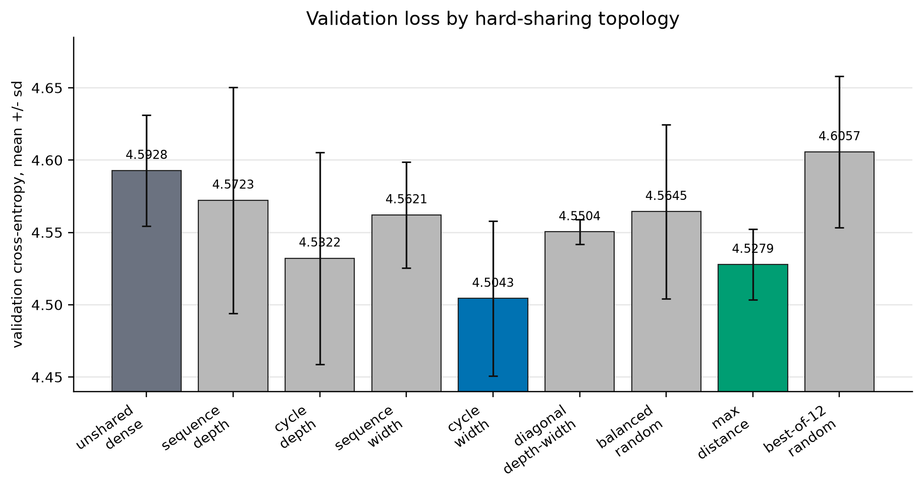
Lower validation CE is better. Error bars and standard deviations are across the three final seeds.

Table 1. Final validation losses. All shared variants use 128 hard-shared MLP blocks and 67.1M MLP-bank parameters. The unshared model is the practical dense baseline.

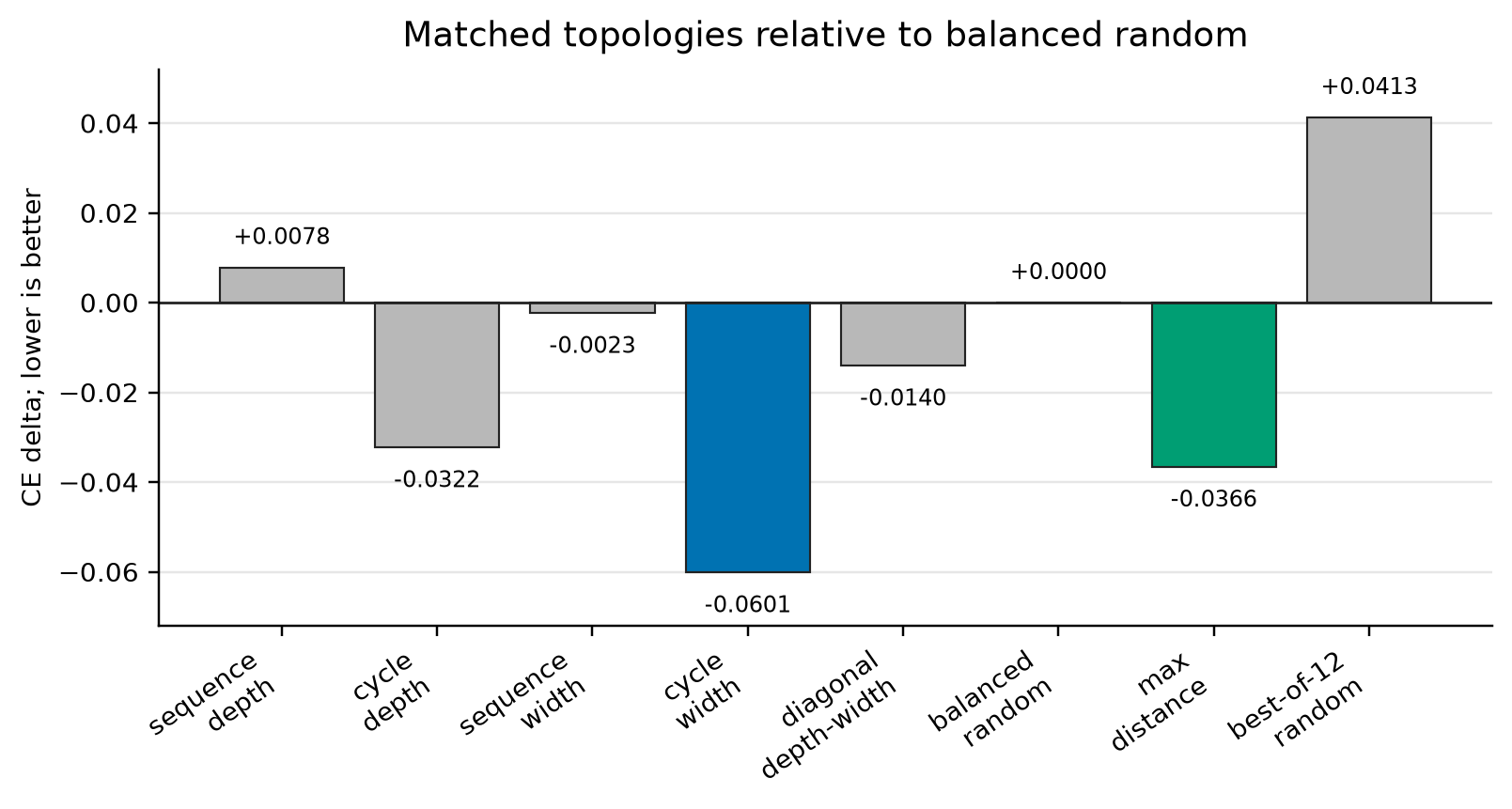
The result in Table 1 is that topology changes loss at fixed parameter count. Cycle width sharing beats balanced random by 0.0601 CE and beats the unshared dense baseline by 0.0885 CE in this training budget. Maximum-distance sharing also beats balanced random by 0.0366 CE, which supports the maximum-distance hypothesis as a useful constraint. It is not the best tested topology.

The searched random result is informative because it failed in the final comparison. The best proxy layout among 12 random candidates had 5.6940 proxy validation CE after 800 steps, but the final three-seed mean was 4.6057. The search procedure did not discover a topology that beat the regular width-sharing rule.

5. What cycle width sharing is

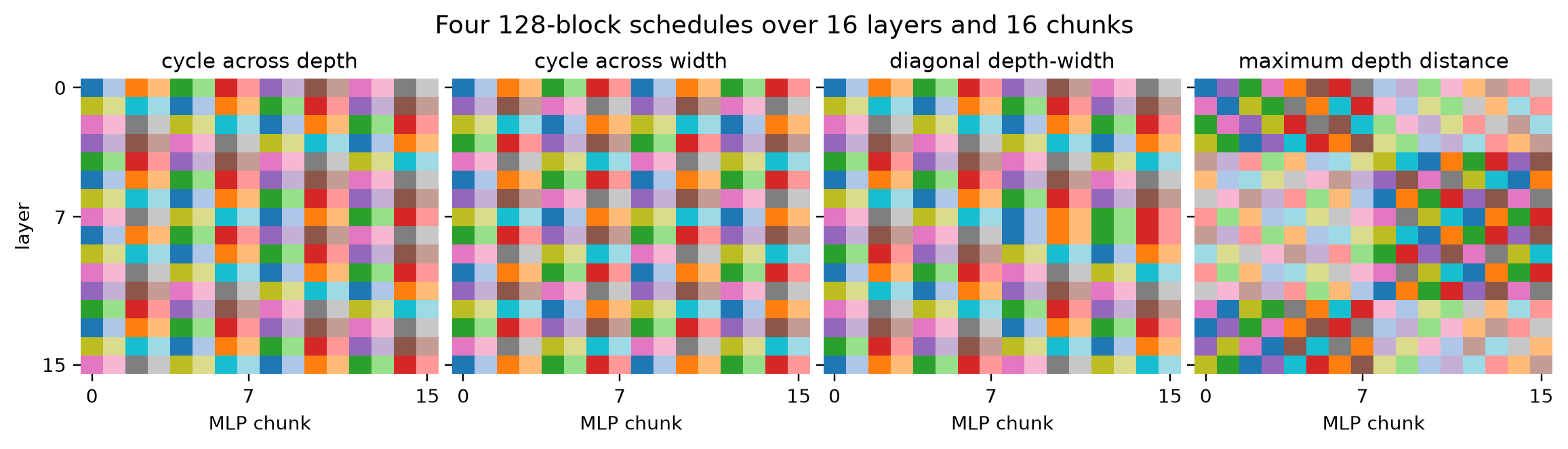
Cycle width sharing keeps each layer’s MLP block bank separate. With 16 layers and 128 shared blocks, each layer receives 8 learned blocks. The schedule is

\[ a_{\mathrm {width\ cycle}}(\ell ,c)=8\ell +(c\bmod 8). \]

Thus, within a layer, chunks 0 and 8 share a block, chunks 1 and 9 share a block, and so on. No block is shared across two different layers.

This comparison matters because the parameter count is identical to the depth-sharing and random-sharing variants. Cycle width sharing is not larger. It chooses a different reuse topology.

The cycle-vs-sequence distinction should be interpreted cautiously. MLP chunk order is an implementation convention. Sequence width and cycle width are both width-axis sharing rules, and they differ less conceptually than width sharing differs from depth sharing. The stable conclusion concerns the axis. Sharing across width works better than sharing across depth.

6. Interpretation

Depth and width are not equivalent axes. Depth is an ordered computation. A lower layer and an upper layer see different residual-stream distributions, serve different roles, and operate at different stages of abstraction. Tying a block across depth forces one operator to act in multiple computational regimes.

Width inside the MLP is more exchangeable. A feedforward layer expands the residual stream into many hidden channels, applies a nonlinearity, and projects back. The hidden chunks are parallel contributors to the same layer update. Sharing there removes degrees of freedom, but it preserves the layer-specific transformation.

This interpretation explains the ordering. Sequence depth sharing performs poorly because adjacent layers are tied. Cycle depth sharing improves when tied uses are separated by 8 layers. Maximum-distance sharing improves further over random because it explicitly pushes tied uses apart. Cycle width sharing has the lowest loss because it avoids cross-depth tying altogether.

This revises the original interpretation of the experiment. The best hand-designed irregular-style topology, maximum depth distance, is strong. The winning rule is simpler. Keep depth distinct, share width.

7. Relation to CNNs and structured matrices

The same axis principle appears in convolutional networks. CNNs share a kernel across spatial positions because the same local feature can appear at different image locations ( LeCun et al. 1998). Depthwise separable convolutions and MobileNets further separate spatial and channel mixing, showing that the axis of reuse is a core architectural decision rather than a bookkeeping detail ( Howard et al. 2017).

The same principle appears in structured matrices. ACDC, Fastfood-style layers, tensor-train layers, butterfly matrices, Butterfly Transform, Monarch matrices, and Monarch Mixer all replace dense width mixing with structured reuse patterns ( Sindhwani et al. 2015, Yang et al. 2014, Novikov et al. 2015, Dao et al. 2019, Alizadeh-Vahid et al. 2019, Dao et al. 2022, Fu et al. 2023). Recent structured-matrix work also finds that different structured replacements need different optimization settings, which reinforces that the structure is an architectural choice, not a neutral parameter-count reduction ( Qiu et al. 2024).

The experiment here adds a direct Transformer result to that picture. When hard sharing is forced, width-axis reuse is the most reliable topology among the tested alternatives. CNNs share across image width and height because those axes repeat local roles. Structured matrices share across width because width mixing contains reusable algebraic structure. Transformer MLPs show the same pattern: share along the redundant axis before sharing along the ordered computational axis.

Conclusion

At a fixed hard-sharing budget, parameter-sharing topology decides model quality. In this 16-layer, width-1024 Transformer LM, cycle width sharing was the best tested topology, maximum-depth-distance sharing was a strong but secondary result, and random layout search did not beat the regular width rule.

The resulting design rule is simple: if a Transformer MLP must reuse exact blocks, preserve depth first. Different layers serve different purposes, while width chunks inside a layer tolerate reuse. That is the transferable topological result.

References

1. Reza Alizadeh-Vahid et al.  Butterfly Transform: An Efficient FFT Based Neural Architecture Design. CVPR 2020.
2. Tri Dao et al.  Learning Fast Algorithms for Linear Transforms Using Butterfly Factorizations. ICML 2019.
3. Tri Dao et al.  Monarch: Expressive Structured Matrices for Efficient and Accurate Training. ICML 2022.
4. Mostafa Dehghani et al.  Universal Transformers. ICLR 2019.
5. Daniel Y. Fu et al.  Monarch Mixer: A Simple Sub-Quadratic GEMM-Based Architecture. NeurIPS 2023.
6. Aaron Gokaslan and Vanya Cohen. OpenWebText Corpus. 2019.
7. Andrew G. Howard et al.  MobileNets: Efficient Convolutional Neural Networks for Mobile Vision Applications. 2017.
8. Zhenzhong Lan et al.  ALBERT: A Lite BERT for Self-supervised Learning of Language Representations. ICLR 2020.
9. Yann LeCun et al.  Gradient-Based Learning Applied to Document Recognition. Proceedings of the IEEE 1998.
10. Alexander Novikov et al.  Tensorizing Neural Networks. NeurIPS 2015.
11. Alec Radford et al.  Language Models are Unsupervised Multitask Learners. OpenAI 2019.
12. Siddharth Sindhwani et al.  ACDC: A Structured Efficient Linear Layer. 2015.
13. Sho Takase and Shun Kiyono. Lessons on Parameter Sharing across Layers in Transformers. 2021.
14. Ashish Vaswani et al.  Attention Is All You Need. NeurIPS 2017.
15. Yinchong Yang et al.  Deep Fried Convnets. ICCV 2015.
16. Yifan Qiu et al.  Compute Better Spent: Replacing Dense Layers with Structured Matrices. ICML 2024.